

عاشق یادگیری
هوش مصنوعی برای تشخیص بیماری (بخش سوم)
در این بخش میخواهیم به معرفی عملیات پیش پردازش بر روی تصاویر بپردازیم.
پیشپردازش تصاویر در کراس
ما قبل از آموزش مدل باید تصاویر را به گونه اصلاح کنیم که برای آموزش در شبکه های عصبی کانولوشن مناسب باشند به همین خاطر از تابع ImageDataGenerator در کتابخانهی کراس استفاده میکنیم که عملیات preprocessing و data augmentation را برای ما انجام میدهد.
# Import data generator from keras
from keras.preprocessing.image import ImageDataGenerator
# Normalize images
image_generator = ImageDataGenerator(
    samplewise_center=True, #Set each sample mean to 0.
    samplewise_std_normalization= True # Divide each input by its standard deviation
)استانداردسازی
در کدهای بالا ما مقدار میانه تصاویر را برابر ۰ و مقدار انحراف معیار تصاویر را برابر ۱ قرار دادیم. به یه بیان دیگه میشه گفت که ما مقادیر جدیدی رو به هر پیکسل از تصویر دادیم که اون مقدار جدید از معادلهی زیر محاسبه میشه
(x-μ)/σ
که در اینجا x مقدار فعلی پیکسل هست و σ انحراف معیار و μ میانهی پیکسلهای تصاویر است.
در کدهای زیر سایز تصاویر را به عنوان ورودی های شبکهی عصبی کانولوشن کاهش میدهیم برای اینکه روند آموش سریعتر انجام شود
# Flow from directory with specified batch size and target image size
generator = image_generator.flow_from_dataframe(
dataframe=train_df,
directory="nih/images-small/",
x_col="Image", # features
y_col= ['Mass'], # labels
class_mode="raw", # 'Mass' column should be in train_df
batch_size= 1, # images per batch
shuffle=False, # shuffle the rows or not
target_size=(320,320) # width and height of output image
)خوب حالا تصویر اول دیتاست رو رسم میکنیم و باهم میبینیم که چه تغییراتی در تصویر ایجاد شده
# Plot a processed image
sns.set_style("white")
generated_image, label = generator.__getitem__(0)
plt.imshow(generated_image[0], cmap='gray')
plt.colorbar()
plt.title('Raw Chest X Ray Image')
print(f"The dimensions of the image are {generated_image.shape[1]} pixels width and {generated_image.shape[2]} pixels height")
print(f"The maximum pixel value is {generated_image.max():.4f} and the minimum is {generated_image.min():.4f}")
print(f"The mean value of the pixels is {generated_image.mean():.4f} and the standard deviation is {generated_image.std():.4f}")خروجی قطعه کد بالا به صورت زیر است
The dimensions of the image are 320 pixels width and 320 pixels height
The maximum pixel value is 1.7999 and the minimum is -1.7404
The mean value of the pixels is 0.0000 and the standard deviation is 1.0000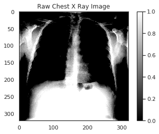
حال به مقایسهی توزیع مقادیر پیکسلها در تصویر اصلی و تصویر اصلاح شده میپردازیم
# Include a histogram of the distribution of the pixels
sns.set()
plt.figure(figsize=(10, 7))
# Plot histogram for original iamge
sns.distplot(raw_image.ravel(),
             label=f'Original Image: mean {np.mean(raw_image):.4f} - Standard Deviation {np.std(raw_image):.4f} \n '
             f'Min pixel value {np.min(raw_image):.4} - Max pixel value {np.max(raw_image):.4}',
             color='blue',
             kde=False)
# Plot histogram for generated image
sns.distplot(generated_image[0].ravel(),
             label=f'Generated Image: mean {np.mean(generated_image[0]):.4f} - Standard Deviation {np.std(generated_image[0]):.4f} \n'
             f'Min pixel value {np.min(generated_image[0]):.4} - Max pixel value {np.max(generated_image[0]):.4}',
             color='red',
             kde=False)
# Place legends
plt.legend()
plt.title('Distribution of Pixel Intensities in the Image')
plt.xlabel('Pixel Intensity')
plt.ylabel('# Pixel')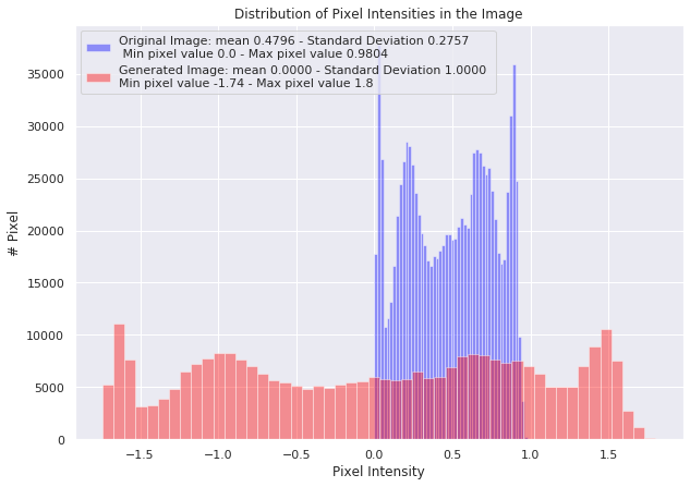
مطلبی دیگر از این انتشارات
هوشمصنوعی برای تشخیص بیماری (بخش دوم)
مطلبی دیگر از این انتشارات
هوش مصنوعی برای تشخیص بیماری (بخش پنجم)
مطلبی دیگر از این انتشارات
هوش مصنوعی برای تشخیص بیماری (بخش اول)